1995issue C111-11
Constructing scaled z-score normalization for model inputs
Forecast models that work best on a limited numeric range often first map unbounded ordered observations through a bounded preprocess. A scaled z-score built from an explicit lookback window keeps the original density visible, rather than letting a sigmoid map flatten the tails.
- Forecast models that work best on a limited numeric range often first map unbounded ordered observations, such as prices, through a bounded preprocess.
- Common sigmoid maps send an input into a unit interval, but variation outside a narrow raw band collapses to the bound and most of the original price variation disappears.
- Z-score normalization subtracts the lookback mean and divides by the lookback standard deviation; dividing those scores by 3 places about 98.9 percent of values inside -1 to +1.
- The scaled dimensionless scores keep the original density shape and the actual sample extremes, and they can be compared across series whose raw price levels differ widely.
Bounded inputs for forecast models
Forecast models that work best on a limited numeric range often first map unbounded ordered observations, such as prices, through a bounded preprocess. That preprocess is a squashing function: it maps an unbounded series onto a limited numeric range before the values enter the model.
Two common sigmoid maps send an input into either the interval from -1 to +1 or the interval from 0 to +1. A sigmoid map is an S-shaped bounded transform that saturates at the extremes and can discard remaining variation outside a narrow raw band.
What a sigmoid map discards
In the first of those maps, variation outside about -6.4 to +8 collapses to the bound. In the second, variation outside about -16 to +16.9 is lost.
On a weekly closing-price sample from March 14, 1986 to May 4, 1994, raw values ran from 3.222 to 92.50, with a mean of 38.190 and a standard deviation of 31.262. After those S-shaped maps were applied to the same weekly closes, the transformed series no longer displayed most of the original price variation.
Building the scaled z-score
Z-score normalization is constructed by subtracting the sample mean from each observation and dividing by the sample standard deviation. Subtract the lookback mean from each ordered observation and divide by the lookback standard deviation.
An interval from -3 to +3 is described as holding about 98.9 percent of the standardized observations, so dividing each z-score by 3 yields a series with mean zero, standard deviation about 0.333, and about 98.9 percent of values inside -1 to +1.
The probability density of the scores divided by 3 keeps the same shape as the original series, and the plotted extremes remain the actual sample extremes. The optional rescale is only a further division so most of the mass sits inside a chosen interval.
The lookback window and dimensionless scores
The construction requires an explicit lookback window, the defined sampling interval over which the mean and standard deviation are estimated. The resulting values are dimensionless scores: unit-free standardized numbers that let series with very different raw scales be compared on the same numeric footing, including series whose raw price levels differ widely.
Sigmoid maps versus scaled z-score on the printed Microsoft closes
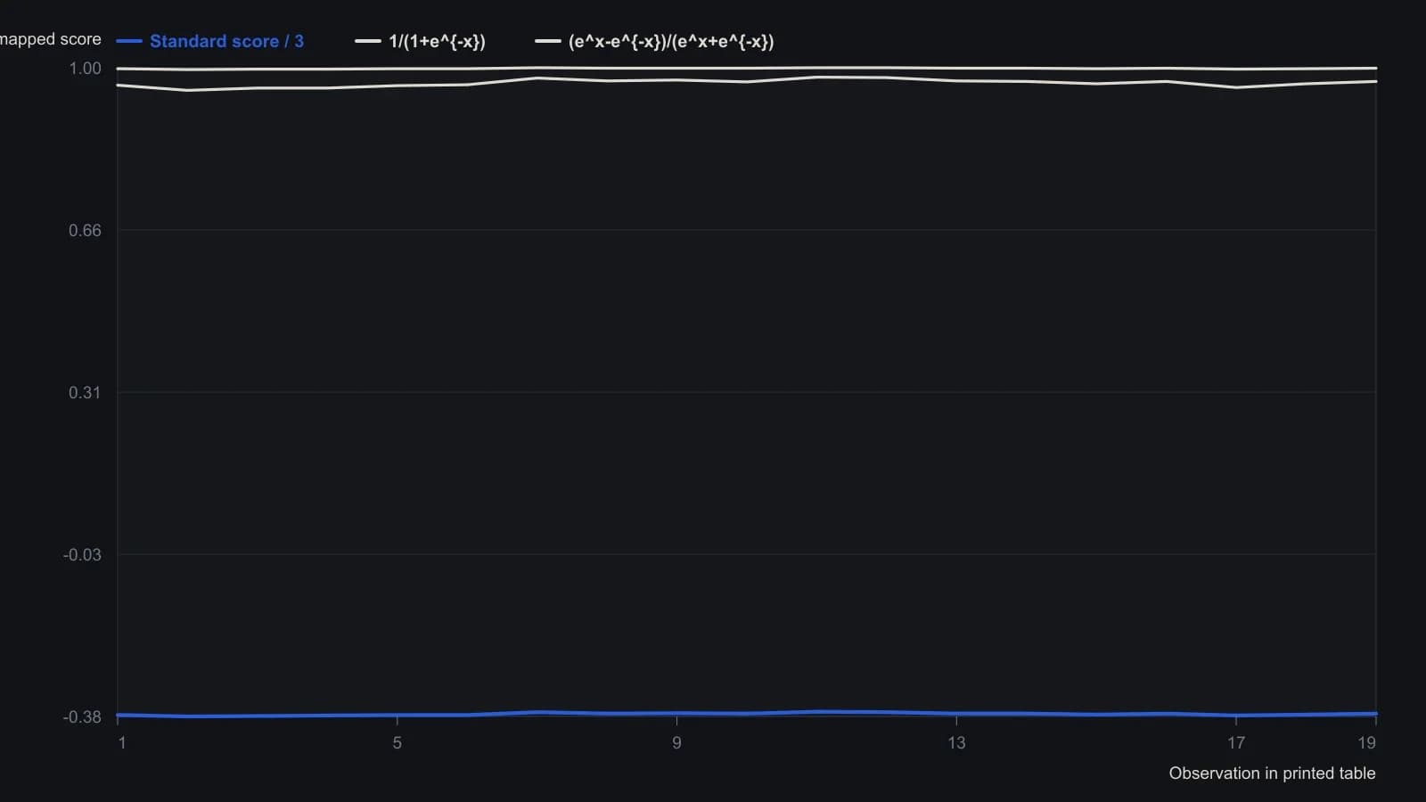
The printed z-scores use the mean and standard deviation of the longer Microsoft sample, so these early closes near 3 all land around −1.1 before the divide-by-3 scale.
All readings on this track · 11 readings
- 1991Constructing standardized sentiment trend filters
- 1995Market z-score residuals for style pair construction
- 1995Constructing scaled z-score normalization for model inputs
- 1996Normalize price and volume onto a common scale
- 2001Constructing pair spreads with z-score triggers
- 2003Rebuilding band distance as a z-score crossover
- 2003Constructing price z-scores with dual averages and bands
- 2003Zigzag target zones from a normalized deviation oscillator
- 2005Constructing a z-score scored range-breakout filter
- 2006Constructing a trend system from Bollinger Bands and z-scores
- 2011How an adjustable-bands z-test resizes the no-trade zone