1993issue C091-3
A twelve-month moving-average filter for inflation direction
This archive lesson specifies a two-input monthly filter: subtract capacity utilization and the unemployment rate from their own twelve-month simple moving averages, invert and scale the labor term so the two deviations share weight, and read only the sign of the combined series as a directional forecast of the inflation rate.
- Fix a monthly sampling interval and subtract each cost-pressure series from its own twelve-month simple moving average.
- Multiply the unemployment deviation by negative two and a half so the labor term is inverted and given comparable weight to the capacity-utilization deviation.
- Read only the sign of the combined series: above zero forecasts a rise in the inflation rate from its then-current level, and below zero forecasts a fall.
- The construction is a directional forecast of the year-over-year consumer-price rate, not a forecast of the inflation level.
Two monthly cost-pressure inputs
The filter is assembled from two monthly inputs, capacity utilization and the unemployment rate. Each series is subtracted from its own twelve-month simple moving average, the unweighted mean of the latest twelve monthly observations of that series, used as the local baseline subtracted from the current reading.
Capacity utilization and unemployment are used as stand-ins for materials-market and labor-market cost pressure, the two primary cost channels named in the construction.
Lookback, inversion, and equal-weight scale
The capacity-utilization deviation is the gap between the current capacity-utilization rate and its twelve-month simple moving average. That gap stands in for materials-market cost pressure.
The scaled-unemployment oscillator is the gap between the unemployment rate and its twelve-month simple moving average, multiplied by negative two and a half. That step inverts the labor term and gives it comparable weight to the capacity-utilization deviation.
The sampling interval is monthly and the lookback is twelve months. Editorial: the lookback, the inversion, and the equal-weight scale are the construction contract that lets the filter be rebuilt as an explicit baseline.
How to read the signed inflation filter
The two deviations are combined into a monthly signed inflation filter. Editorial: only the sign of that sum is read as the forecast.
A reading above zero is interpreted as a forecast that the inflation rate will rise from its then-current level. A reading below zero is interpreted as a forecast that the rate will fall.
The constructed series is presented as a directional forecast of the inflation rate, not as a forecast of the inflation level itself. Inflation in the comparison is measured as the year-over-year consumer-price rate, the percentage change in the Consumer Price Index versus the same month a year earlier.
Comparison overlay and stated leads
Unemployment is inverted on the comparison chart so its peaks and troughs can be aligned visually with capacity utilization and the inflation rate. Capacity utilization and unemployment are described as tending to turn before the inflation rate.
The illustrated overlay advances the constructed series by six months. The notes give an average lead versus the consumer-price trend of seven to nine months, and a shorter five-to-seven-month lead in the later decade of the sample.
Inflation indicator shifted six months versus CPI
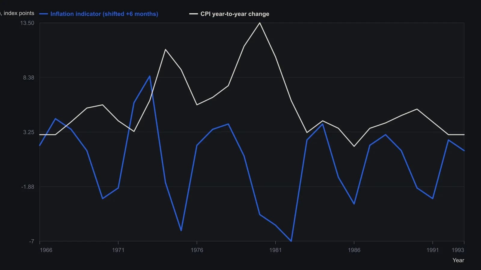
The source shifts the indicator forward six months on this chart. Axis labels on the scan are inverted; y-values are the printed scale units, sampled coarsely because the raster cannot support finer precision.
All readings on this track · 15 readings
- 1990Building a percent-difference moving-average oscillator
- 1991Ease of movement oscillator construction
- 1993A twelve-month moving-average filter for inflation direction
- 1993Constructing two-endpoint JSA moving averages
- 1999Centered moving averages for trend construction
- 2000Constructing a slope-corrected moving average
- 2000Lookback length as a construction check for the modified moving average
- 2001Smoothing balance of market power with a moving average
- 2005Three-state moving-average directional breakout construction
- 2005Constructing a move-adjusted moving average
- 2005Moving-average construction: windows, weights and stops
- 2008Constructing stacked moving-average filters
- 2011Constructing percentage-offset moving-average bands
- 2015Linearity, commutation, and ratio smoothing in moving averages
- 2019Constructing a 50-200 sma-channel for swing entries and exits