1982issue C021-3
Constructing moving averages with weights, alignment, and adaptive lookbacks
Build an equal-weight moving average from a lookback of N observations, then change the window weights, the plot location, and whether that lookback stays fixed.
- A simple moving average chooses a lookback N, averages the last N successive observations, and places that value on the last day of the window.
- The three construction variables are the number of days in the window, the weighting scheme inside that window, and the plot location relative to the original data.
- A centered plot is described as the better historical fit and trails the latest observation by half the window, while a later day is suggested as a possibly better forecast placement.
- A fixed lookback is described as unlikely to remain appropriate indefinitely, and an adaptive filter that searches a shifting lookback is reported as computationally heavy.
Three construction variables
The archive identifies three construction variables: the number of days in the window, the weighting scheme inside that window, and the plot location relative to the original data.
A lookback is the count N of successive price, volume, or breadth observations inside one average. Plot location is where the computed average is drawn relative to the original series, choosing historical fit or a forecast horizon.
Equal-weight construction
A moving average is the equal-weight mean of the last N ordered observations, used as a smoother or as a one-step forecast. A simple moving average is built by choosing a lookback N, averaging the last N successive observations, and placing that value on the last day of the window.
In the equal-weight case the only explicit design choice is N. Characteristic lengths are described as instrument-specific, without an agreed method for choosing or testing them. The worked construction uses a five-day window, and the same procedure is stated to apply for any chosen N.
A recursive one-step forecast
One forecasting extension plots the latest average one day ahead, then forms the next forecast by dropping the oldest observation and inserting the first projected value.
That recursive forecast is characterized as more suitable after sideways prices and as lagging a rising or falling series.
Unequal weights in the same window
A weighted moving average keeps the same lookback window with unequal coefficients so some observations contribute more than others. Each day need not contribute an equal share.
Suitable weights are sought by testing trial values against the next realized observation and then adjusting them.
Centered plot and later placement
A centered plot aligns the average at the midpoint of its window. It follows the historical path but delays the latest reading by half the lookback.
For N equal to 5, a centered average is plotted on the third day, is described as the better historical fit, and trails the latest observation by half the window. A later day, such as the fourth, is suggested as a possibly better forecast placement.
A shifting lookback
A fixed N is described as unlikely to remain appropriate indefinitely. An adaptive filter is a search that lets the averaging length or weights change when a fixed lookback no longer matches recent data.
Automatically assessing a shifting lookback with an adaptive filter is reported as computationally heavy, with a first program run taking almost four hours.
Days of history consumed by CompuTrac moving-average studies
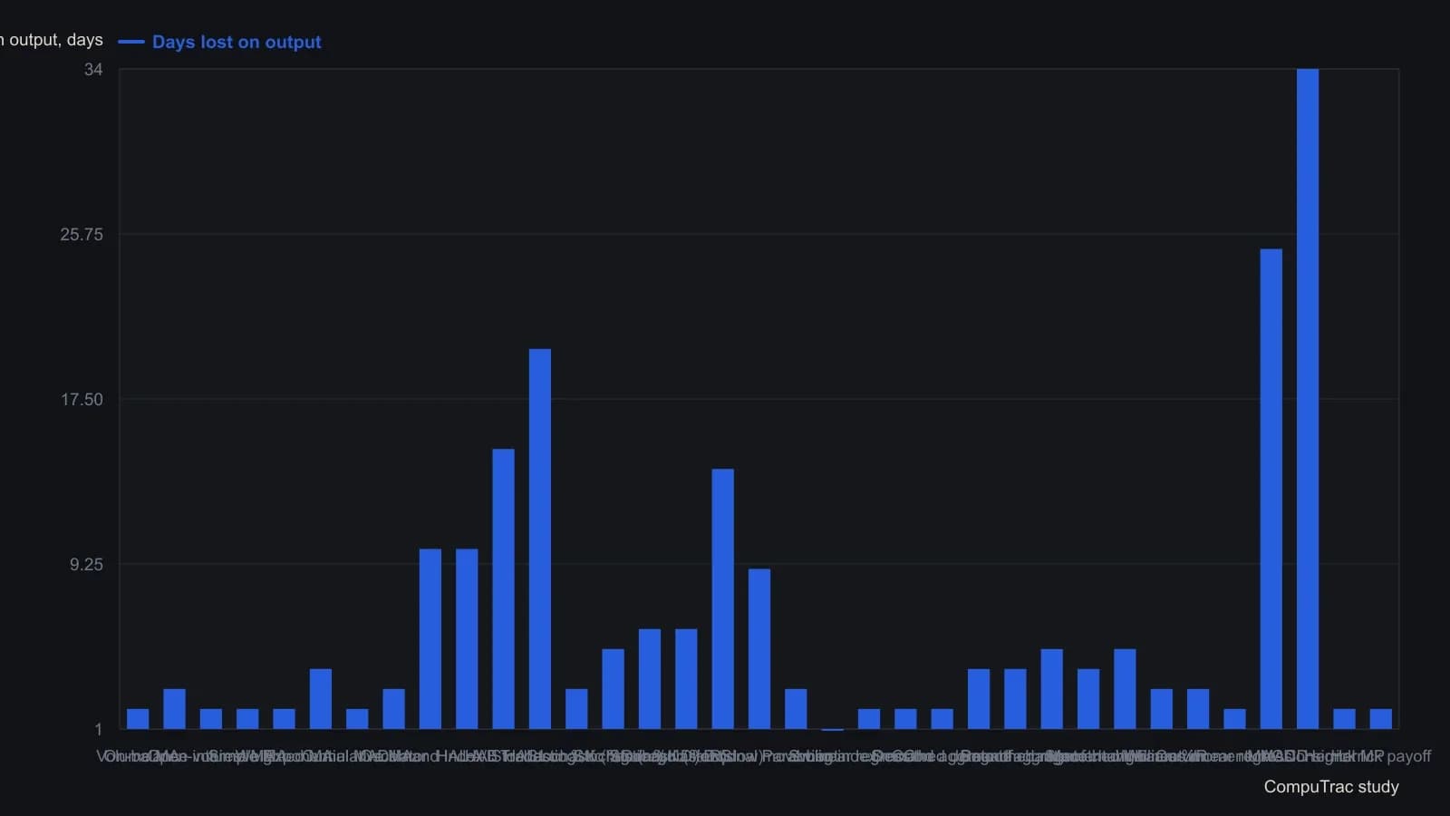
Example input lengths in the source are demonstration settings, often a 3-day window, not recommended defaults. Rows marked not a moving average, undetermined, or without a numeric days-lost figure were omitted.
All readings on this track · 9 readings
- 1982Constructing moving averages with weights, alignment, and adaptive lookbacks
- 1990Constructing adaptive filters from equal-weight averages
- 2000Cycle-scaled lookbacks for a channel-breakout rule
- 2000When charting code breaks the adaptive trendline
- 2001Nonlinear Ehlers filter construction from momentum and distance weights
- 2001How a fixed smoother becomes a living parameter surface
- 2005A three-part workshop for adaptive-filter length search
- 2010Rebuilding an exponential average as a bounded error-correcting filter
- 2018Assembling a recursive median oscillator as a two-stage adaptive filter