2008issue C071-4
Constructing singular-spectrum forecast baselines
An embedded price window can be turned into ranked spectral components and then into a one-step forecast. That forecast is recorded bar by bar and placed beside a same-length exponential moving average that only filters.
- An observed market series can be treated as a slow trend, an oscillation whose period and amplitude may change, and a residual random component, and singular spectrum analysis forms those parts from the series itself.
- The construction embeds consecutive segments into a trajectory matrix, groups selected principal components, and uses diagonal averaging to reconstruct trend, periodic structure, or a reduced residual.
- The free parameters are series length, window length, and retained-component count; a historical reconstruction overlay is not a valid out-of-sample reading.
- A forecasting variant records the first projected point of each bar and can be placed next to a same-length exponential moving average that only filters.
Treat the observed series as three parts
An observed market series can be treated as the combination of a slow trend, an oscillation whose period and amplitude may change, and a residual random component. Spectral analysis is a data-adaptive decomposition of that ordered series into trend, oscillatory, and residual parts taken from the singular structure of a trajectory matrix rather than from a fixed trigonometric basis.
Singular spectrum analysis forms its components from the observed series itself. It does not require a preliminary stabilization step or a fixed sine-cosine basis.
Embed consecutive segments
The construction begins by embedding consecutive segments of length m into a trajectory matrix so that repeatable structure in the original series is inherited by those segments. Window length is the spatial dimension m that sets how long each embedded segment is and how narrow the implied reconstruction filter becomes.
Choose series length, window length, and component count
The free parameters are series length N, window length m, and retained-component count L. Increasing m narrows the implied reconstruction filter.
For unknown periods a common choice is m equal to half the sample length. When a period is known, N is made divisible by that period and m is set to match it.
Rank the leading components
Leading components may be kept when their eigenvalues exceed one, or by reading breaks on a descending eigenvalue chart. Component count is the number L of leading singular components retained for reconstruction or forecast after that numerical or graphical cutoff.
In a 240-minute EUR/USD illustration with N equal to 50 and m equal to 25, the first singular value was taken as the trend. Slope changes were used to cap L near 23 to 25, and a working set of 3 to 10 components was described as often adequate.
Reconstruct with diagonal averaging
After grouping selected principal components, diagonal averaging reconstructs a series that can isolate trend, recover periodic structure, or reduce the residual. That step converts a grouped low-rank trajectory matrix back into a single reconstructed series.
Record the first projected point
Because the reconstructed path is recomputed as new bars arrive, a historical overlay of that path is not a valid out-of-sample reading. A forecasting variant instead records the first projected point of each bar. That forecasting moving SSA line can be placed next to a same-length exponential moving average that only filters.
Exponential smoothing is a recursively weighted average of ordered prices used as that same-length, filtration-only counterpart. A moving average is the same-length filtration of ordered prices used as a non-forecasting baseline against which a reconstructed or projected spectral smoother can be compared.
One-step SSA forecast against a matching EMA on 4-hour EUR/USD
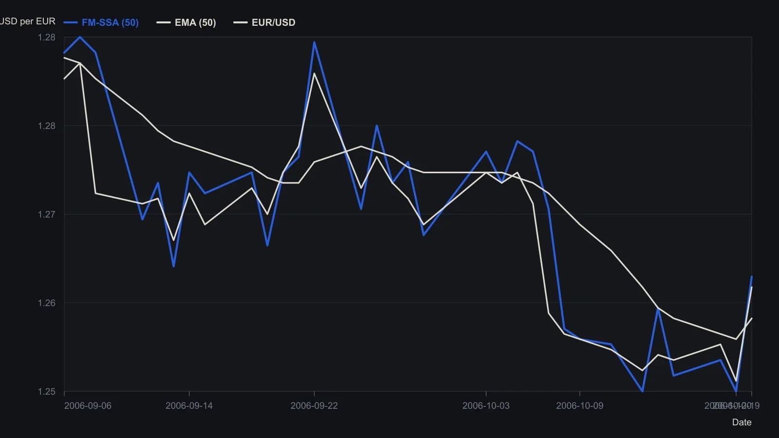
Source overlay is SSA with series length 50, window 25 and components 1–3 on the close; the EMA length is 50. Day-of-month labels wrap at a month-end and were assigned as 6 September–20 October 2006 from those labels plus the 25 December 2006 workspace stamp. Expect about one pip of reading error.
When a linear generating model is too restrictive
The linear form of the construction assumes a linear generating model. Kernel methods were introduced when that assumption was treated as too restrictive for market series.
All readings on this track · 21 readings
- 1982Spectrum-first construction of moving-average trend filters
- 1990Crowd questions that switch cycle regimes
- 1993Antithetic twins to cancel origin-linked forecast bias
- 1994Constructing frequency response from a three-stage filter cascade
- 1994Bench-testing smoothers with cycle phase and power
- 1995Constructing minimum tradable cycles from spectral noise
- 1995Spectral whipsaw limits for a price-crossing average
- 1996Constructing market phase from dominant-cycle components
- 2000Constructing a Hilbert squelch dominant-cycle gate
- 2007When cycle mode fails: regime gates for spectral trades
- 2008Constructing singular-spectrum forecast baselines
- 2008Stacking a midband cycle gate on a short-memory trend filter
- 2011Engineering spectral cycle detection and moving-average harmony
- 2011Evaluating fixed oscillators against a moving dominant cycle
- 2011A construction checklist for a dominant-cycle sinewave
- 2012Assembling a market-mode heatmap from successive band-pass filters
- 2012Adaptive trend detection from dominant-cycle spectra
- 2015Constructing price paths from cycles and support
- 2018Oscillator distribution shape for mean-reversion filters
- 2020Constructing a cosine-correlation cycle and phasor trend filter
- 2020Constructing a correlation-cycle market-state engine