1994issue C091-3
Constructing labeled cycle lengths from FFT spectra
An ordered price window is decomposed with a fast Fourier transform and displayed as a Fourier power spectrum. Spectral analysis then converts each strong bar from cycle frequency into a labeled cycle length before that peak is judged as a forecast input.
- An ordered price series can be treated as a composite waveform whose irregular spacing between successive highs and lows is the visible sum of cycles with unequal lengths.
- A fast Fourier transform produces a Fourier power spectrum of cycle power versus frequency, and spectral analysis converts each strong bar into a cycle length.
- The dominant frequency is the highest-power peak after the zero-frequency bar, and a trigger frequency can be read from a neighboring pair of histogram bars.
- Construction requires a detrended window that does not contain a major trend reversal, because residual drift can dominate the spectrum and a reversal can be recovered as an extra cycle.
What the construction produces
Fourier analysis treats an ordered market series as a sum of cycles and recovers those cycles as frequency components. An ordered price series can be treated as a composite waveform whose irregular spacing between successive highs and lows is the visible sum of cycles with unequal lengths.
A fast Fourier transform is the computational procedure that decomposes that ordered price, volume, or breadth series into frequency bins. Spectral analysis then reads those bins as a power spectrum so each strong bar can be converted into a cycle length.
Prepare the price window
The construction step requires a detrended window that does not contain a major trend reversal. Detrending removes directional drift from the sample so that drift does not dominate the spectrum.
Residual drift can dominate the spectrum. A reversal can be recovered as an extra cycle that the transform will repeat.
Run the fast Fourier transform
A fast Fourier transform decomposes the ordered series into frequency components that can be displayed as a Fourier power spectrum. A Fourier power spectrum is a histogram of cycle power on the vertical axis against frequency on the horizontal axis, starting at zero frequency.
Cycle power is the square of a cycle amplitude. Cycle power equals amplitude squared, so a sine wave with amplitude 2 has power 4.
The spectrum uses as many frequency bars as the smallest power of two that is at least as large as the sample count. That count is the transform length. The first bar is zero frequency, the highest frequency is 180 degrees, and bar i sits at i times 180 divided by that transform length.
Twelve-week sine wave versus phase angle
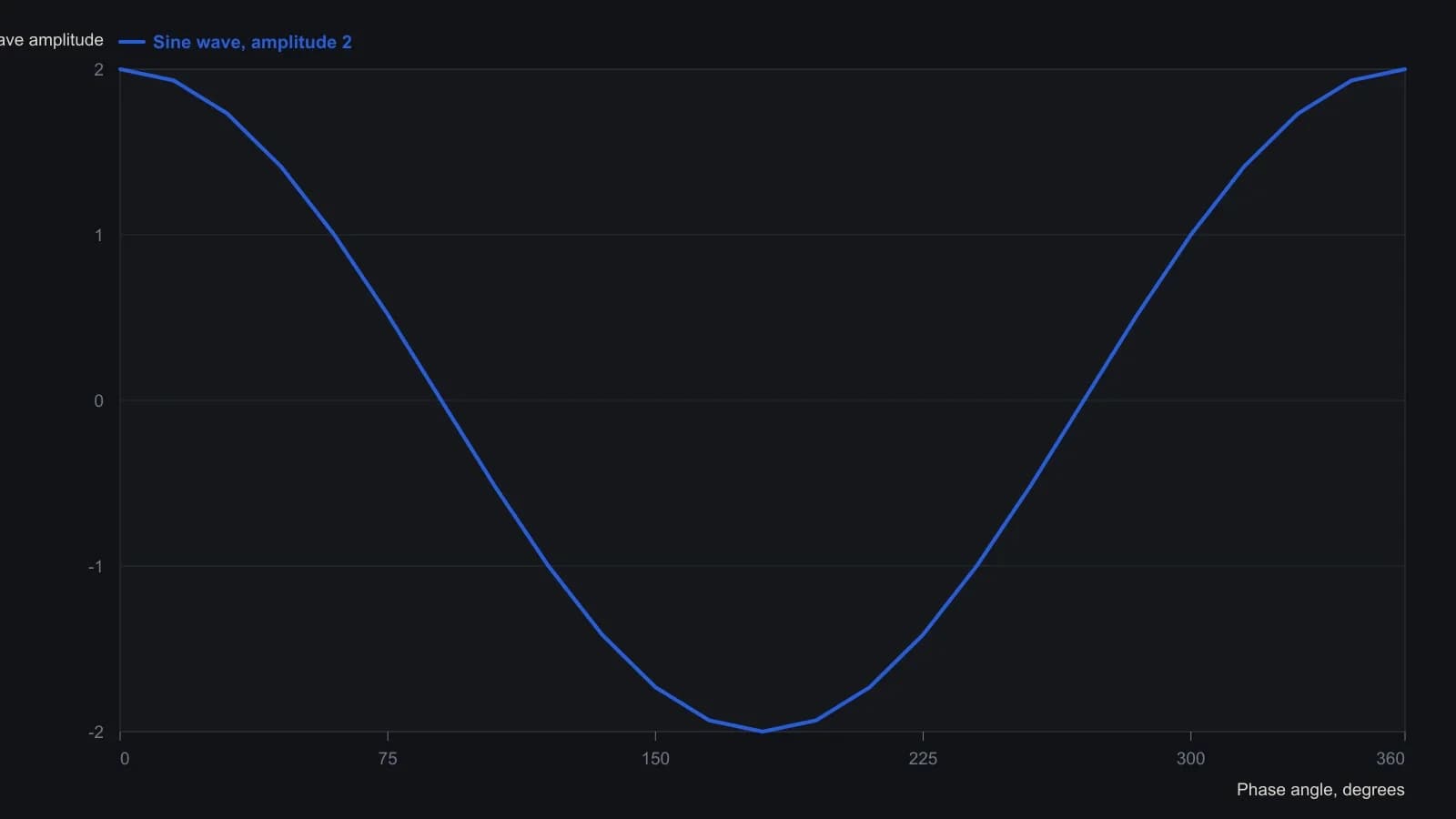
Amplitude is fixed at 2 and cycle length at 12 weeks, so frequency is 30 degrees per week (F = 360/L). The plate is cosine-phased; the sidebar text simply calls it a sine wave.
Read the histogram as cycle lengths
Cycle frequency is phase advance in degrees per sampling period. It is the reciprocal form of cycle length. Frequency in degrees per sample period is 360 divided by cycle length, so a 12-week sine wave advances 30 degrees per week through a full 360-degree cycle.
Spectral analysis uses that conversion to turn each strong histogram bar into a labeled cycle length. The reading order is bin index, then degrees per bar, then cycle length.
Label the dominant and trigger frequencies
In a 71-week window the transform length was 128, and the strongest peak nine bars from zero was read as 13 degrees per week, or 27.69 weeks. That highest-power peak after the zero-frequency bar is the dominant frequency.
A secondary peak between the 20th and 21st bars was assigned the midpoint 20.5 and converted to 29 degrees per week, or 12.5 weeks. That secondary power peak is the trigger frequency.
All readings on this track · 16 readings
- 1982Building FFT spectra to size cycle filters
- 1988Fourier cycle models break in major swings
- 1988Constructing moving average filters from price Fast Fourier Transforms
- 1989Staging Fast Fourier construction under memory limits
- 1993Constructing forecast inputs with moving averages, Fourier transforms and intermarket spreads
- 1994Preprocessing prices so Fourier peaks set moving-average lengths
- 1994Constructing a spreadsheet FFT power spectrum from daily prices
- 1994Building dominant-cycle spectra with FFT preprocessing
- 1994Constructing labeled cycle lengths from FFT spectra
- 1999Fast Fourier Transform reconstruction is not a walk-forward decision tool
- 1999Walk-forward endpoint Fourier construction as a same-day mechanical procedure
- 2002From the power spectrum to indicator windows
- 2003Endpoint Fast Fourier Transform evaluation with walk-forward mechanical rules
- 2004Constructing signal and noise from market waveforms
- 2012A two-stage case study in market cycle analysis
- 2015Whitening pink noise to build a near-zero-lag cycle oscillator