2004issue C111-4
Constructing signal and noise from market waveforms
Assemble an ordered price record as a waveform before any forecast. A wavelet-transform peels a measured residual from a coarser trend, a long moving average can stand in as a carrier-signal, and the same object then sits under a Fourier or spectral baseline.
- Everyday study of market history is framed as a search for a model of later prices, and that premise stays an open hypothesis rather than a closed law.
- A wavelet-transform pair step splits consecutive prices into a coarser trend and a residual noise component that can be dropped, thresholded, or inverted.
- A long moving average can illustrate a carrier-signal, but it mixes noise into that path and does not show whether residual noise is rising or falling.
- Once the record is treated as a waveform, fast-fourier-transform, filters, and related spectral-analysis tools become the next construction options on the same series.
An open hypothesis, not a closed law
Everyday study of market history is framed as a search for a model of later prices. That premise is treated as an open hypothesis rather than a closed law.
Errors in a time series can make a historical test look profitable when no corresponding opportunity was present in the actual path.
Price as a waveform
The construction treats an ordered price record as a waveform. Amplitude is price, a long-horizon economic or yield path is the carrier, and short-lived random deviations are noise.
A moving-average carrier-signal
A 600-day moving average of the Dow Jones Industrial Average from 1970 was used as a simple long-horizon carrier-signal that rolls lesser moves into one smoothed path.
Long moving averages mix noise into the carrier and give no separate reading of whether residual noise inside the series is rising or falling.
DJIA close as a long-term market waveform
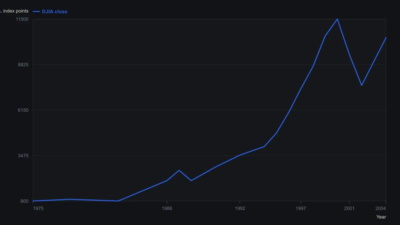
The source uses a 600-day simple moving average as the carrier. On this raster that average appears only as a horizontal last-value line at 10452.8, so its historical path was not digitized. Early-year readings are coarse because the line sits only a few pixels above the baseline.
A pairwise wavelet-transform
A wavelet-transform is a pairwise split of an ordered price series into a coarser trend component and a residual noise component that can be dropped, thresholded, or inverted.
A two-point step on consecutive Nasdaq prints of 1697.8 and 1760.27 produced a trend value of 2445.225 and a noise value of -44.173. Pair-compression repeats that two-point average-and-difference step so each pass leaves half as many values as the pass before.
What to do with the residual
After the wavelet split, residual noise can be dropped, or noise below a chosen threshold can be folded back into the signal by reversing the pair step.
On a normalized-noise series of Nasdaq from November 1998, a high index level did not by itself imply a high noise volume. Normalized-noise expresses the residual as a ratio to the index level so a high price does not inflate the apparent noise volume.
Fourier and spectral options on the same series
Once the record is treated as a waveform rather than a plotted line, a fast-fourier-transform becomes available. Filters and related spectral-analysis tools are the next construction options on the same ordered price, volume, or breadth observations.
All readings on this track · 16 readings
- 1982Building FFT spectra to size cycle filters
- 1988Fourier cycle models break in major swings
- 1988Constructing moving average filters from price Fast Fourier Transforms
- 1989Staging Fast Fourier construction under memory limits
- 1993Constructing forecast inputs with moving averages, Fourier transforms and intermarket spreads
- 1994Preprocessing prices so Fourier peaks set moving-average lengths
- 1994Constructing a spreadsheet FFT power spectrum from daily prices
- 1994Building dominant-cycle spectra with FFT preprocessing
- 1994Constructing labeled cycle lengths from FFT spectra
- 1999Fast Fourier Transform reconstruction is not a walk-forward decision tool
- 1999Walk-forward endpoint Fourier construction as a same-day mechanical procedure
- 2002From the power spectrum to indicator windows
- 2003Endpoint Fast Fourier Transform evaluation with walk-forward mechanical rules
- 2004Constructing signal and noise from market waveforms
- 2012A two-stage case study in market cycle analysis
- 2015Whitening pink noise to build a near-zero-lag cycle oscillator