1994issue C041-3
Constructing a spreadsheet FFT power spectrum from daily prices
A 95-day December copper series from July 8, 1993 through November 18, 1993 is used to show how a linear detrend, a Hanning window, zero-padding to 256 points, and a trading-day axis conversion produce a Fourier power spectrum that can be read by frequency or by cycle length.
- Daily closes were converted to residuals by subtracting a linear least-squares trend before any window was applied.
- A Hanning window tapered those residuals, and the weighted series was the input actually sent to the fast Fourier transform.
- The 95 windowed values were zero-padded to 256 points because the transform length had to be a power of two.
- The same power-spectrum values were plotted against frequency in cycles per year and against cycle length after a 252-trading-day conversion.
A daily series is prepared before the transform
The historical workflow used 95 daily December copper closes running from July 8, 1993 through November 18, 1993. Those ordered closes were not sent straight into a transform. They were first turned into a residual series, tapered with a Hanning window, and zero-padded so the fast Fourier transform could run on a power-of-two length.
Fourier analysis, in this construction, is the decomposition of the prepared observations into sinusoidal components that can then be plotted as a power spectrum. Spectral analysis is the inspection of that power across frequency or cycle length after the preprocessing and the transform. The fast Fourier transform is the discrete mapping into frequency bins once the input length is a power of two.
Remove the linear trend first
Prices were first converted to a residual series by subtracting a linear least-squares trend from each close. The detrend step is that removal of the linear least-squares fit from the price series before windowing.
Apply a Hanning window to the residuals
A Hanning window was built with a one-period increment of 2π divided by the sample count plus one, then applied as 0.5 times one minus the cosine of that increment times the observation index. That raised-cosine weight tapers the ends of the finite sample before the transform.
The window weights were multiplied by the detrended closes to produce the series actually passed to the transform.
Pad to a power-of-two length
The Fourier input and output ranges had to be a power of two, so the 95 windowed values were zero-padded to a 256-point array. Zero-padding means appending zeros so the transform length becomes an admissible power of two.
The same length rule was stated more generally. If the original sample count is below 64 the transform array should be 128 long. If the sample count is between 128 and 256 the array should be 512 long.
Read power on frequency and on cycle length
Each power-spectrum ordinate was the sum of the squared imaginary part and the squared real part of the corresponding complex Fourier bin. That squared magnitude is the vertical axis of the spectrum plot.
Frequency in cycles per year was stepped by 252 divided by 256, matching daily sampling, a 256-point transform, and 252 trading days in a year.
Cycle length was obtained by inverting frequency and multiplying by 252 so the same power values could be plotted against length instead of frequency. Cycle length is the reciprocal of frequency, scaled by the number of trading days in a year when the observations are daily.
December 1993 copper FFT power spectrum
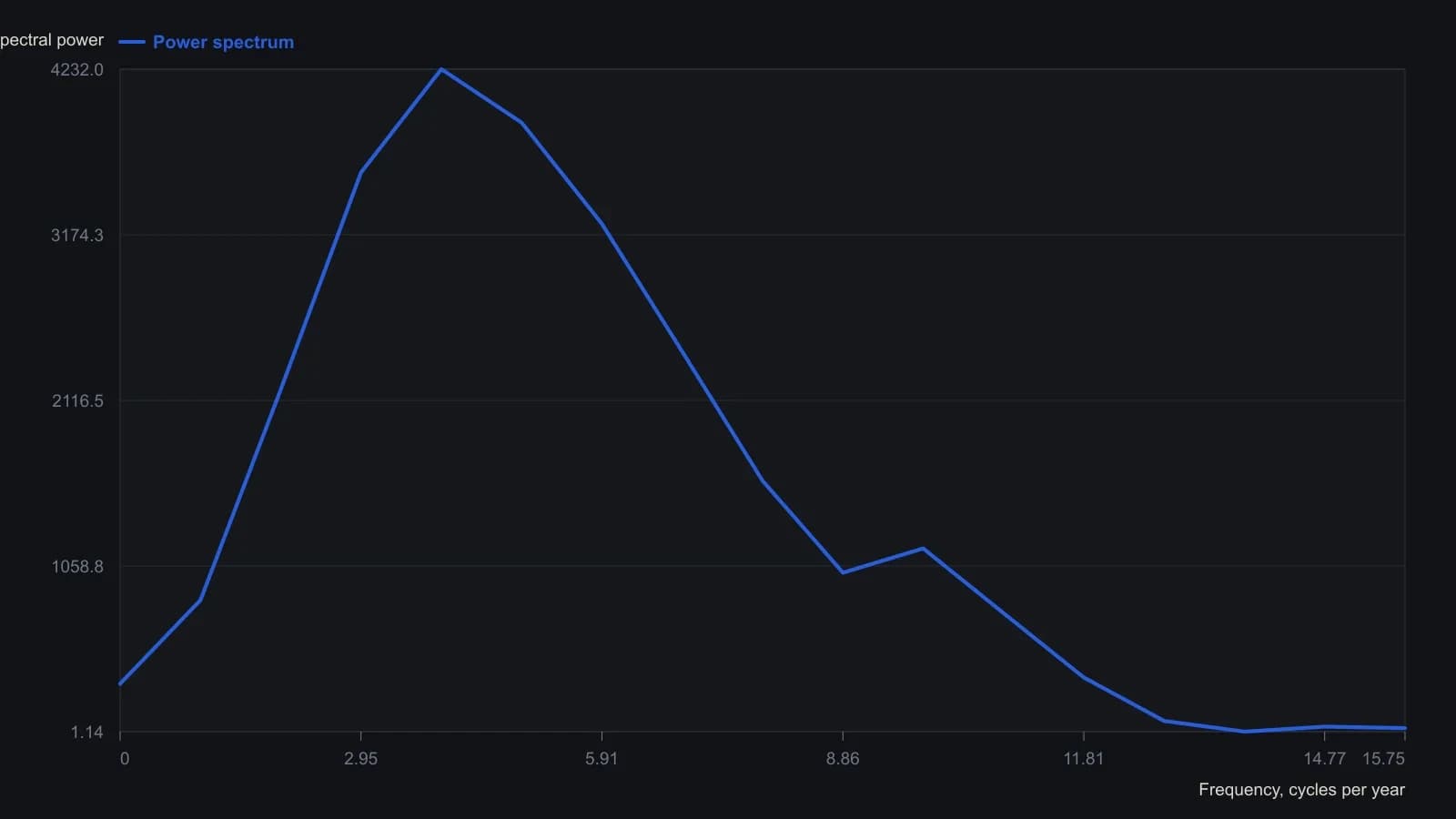
Ninety-five daily closes were linearly detrended, multiplied by a Hanning window, and zero-padded to 256 bins. Frequency is 252 trading days per year divided by the 256-point FFT. Only the lowest 16 bins are visible on the printed sheet.
All readings on this track · 16 readings
- 1982Building FFT spectra to size cycle filters
- 1988Fourier cycle models break in major swings
- 1988Constructing moving average filters from price Fast Fourier Transforms
- 1989Staging Fast Fourier construction under memory limits
- 1993Constructing forecast inputs with moving averages, Fourier transforms and intermarket spreads
- 1994Preprocessing prices so Fourier peaks set moving-average lengths
- 1994Constructing a spreadsheet FFT power spectrum from daily prices
- 1994Building dominant-cycle spectra with FFT preprocessing
- 1994Constructing labeled cycle lengths from FFT spectra
- 1999Fast Fourier Transform reconstruction is not a walk-forward decision tool
- 1999Walk-forward endpoint Fourier construction as a same-day mechanical procedure
- 2002From the power spectrum to indicator windows
- 2003Endpoint Fast Fourier Transform evaluation with walk-forward mechanical rules
- 2004Constructing signal and noise from market waveforms
- 2012A two-stage case study in market cycle analysis
- 2015Whitening pink noise to build a near-zero-lag cycle oscillator