1995issue C021-10
Evaluating mechanical switch rules with a stop-loss order and Sharpe ratio
A historical Mechanical trading system treated entry, cash abstention, and a Stop-loss order as one procedure, then compared that full path with buy-and-hold using a Sharpe ratio instead of isolated indicator stories.
- A ranked 26-week yield-change map was treated as roughly linear, and the extreme tails were used as the informative region for later timing rules.
- A one-rule yield switch, and later a dual-indicator switch, specified buying, moving to cash, and staying out as a single Mechanical trading system.
- A Stop-loss order on the dual-indicator path bounded the largest single loss and the worst peak-to-valley equity drop relative to buy-and-hold.
- A monthly nonannualized Sharpe ratio compared the whole invested-and-cash path with a dividend-preserving buy-and-hold baseline.
Read the switch as one procedure
Editorial interpretation: judge a complete switch as one testable object. Entry, exit, time in cash, and a pre-set loss bound belong to the same Mechanical trading system. The useful comparison is the whole path against buy-and-hold with a Sharpe ratio, not a story about any single indicator.
Yield change ranked against later stock moves
A weekly 26-week percent change in long-term government bond yields was paired with the next 26-week equity-index move. Those pairs were ranked and split into ten equal groups. The pattern was roughly linear: faster yield declines lined up with stronger subsequent stock gains, and faster yield rises lined up with weaker or negative subsequent stock results.
The extreme tails of that yield-change distribution were treated as the most informative region for later timing rules, because turning points in stocks often lined up with periods of rapidly changing rates.
A one-rule yield switch
A one-rule switch bought stocks after a 4% 26-week yield decline and moved to cash after a 14% 26-week yield rise. It was tested on a no-load index fund with dividends reinvested in the market and cash parked in commercial paper, so the buy-and-hold comparison would not drop the dividend stream.
That one-rule procedure stayed in the market 72% of the time from 1980 and 74% of the time from 1957, and every recorded buy signal in those windows was profitable in the backtest.
An adjusted short-sale ratio
A public-to-specialist short-sale ratio was recentered as a 10-week average divided by a 261-week average so that later derivative-era readings could be compared with their own five-year norm rather than with an unadjusted historical scale.
The same ten-group ranking applied to the adjusted short-sale ratio showed subsequent 26-week index gains rising toward the high end of the ratio and falling toward the low end, with the top group near a 24% average annualized gain and the bottom group below 1%.
Two non-price rules, a Stop-loss order, and a Sharpe ratio
A dual-indicator switch combined the two independent, non-price inputs and added a Stop-loss order. That Stop-loss order fired seven times, kept the largest single loss under 4%, and limited the worst peak-to-valley equity drop to 16% in late 1974 versus 45% for buy-and-hold.
Because the dual-indicator procedure was invested only 51% of the time and otherwise earned cash interest, its monthly nonannualized Sharpe ratio was 0.24 against 0.11 for buy-and-hold, or more than twice the tested return per unit of risk.
S&P 500 later return by 26-week bond-yield change
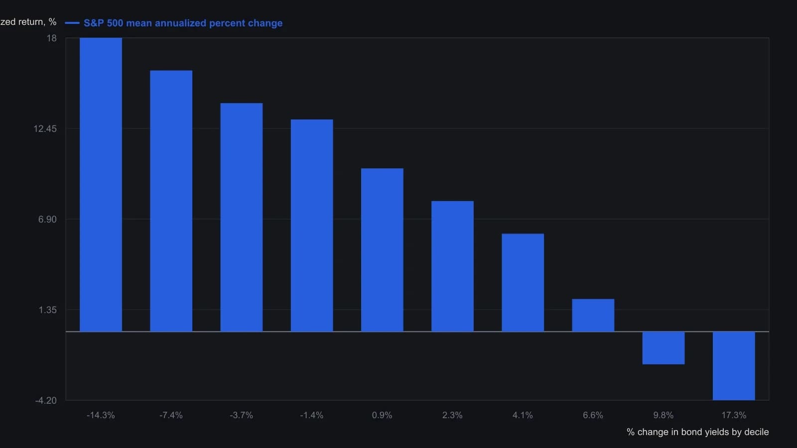
About 1,950 weekly observations from 1957 to mid-1994, ranked by 26-week percent change in the long-term U.S. government bond yield and grouped into ten equal clusters. Each observation is paired with the subsequent 26-week S&P 500 change, shown here as a mean annualized percent change.
All readings on this track · 12 readings
- 1986Auditing stochastic crossovers with moving-average baselines
- 1994Evaluating system changes with chi-square, Sharpe, and leverage
- 1995Evaluating mechanical switch rules with a stop-loss order and Sharpe ratio
- 1995Intermediate-term allocation with drawdown filters
- 1996Evaluating a multi-market book without picking winners
- 1996Regime-aware allocation beyond a single equity trend
- 1997Evaluating managed futures as portfolio diversifiers
- 2008Audit an out-of-the-money covered-call overlay against a Sharpe control
- 2013Constructing the Sharpe ratio as return over variability
- 2014Expected value and bet size are separate controls
- 2015Constructing a Sharpe-style score from profit and loss variability
- 2019Continuous futures series and long-horizon allocation evaluation