1986issue C021-8
Evaluate the price random-walk question as a gated quantile lab
A random-walk hypothesis test asks whether ordered prices came from a process that is both random and independent. This archive article treats that question as a sequence of gates: a split-sample stationarity check, then a quantile and chi-square randomness test, then a finite temporal window for any leftover serial influence.
- A random-walk process is both random and independent, and independence means earlier outcomes do not change the odds of the next outcome.
- Stationarity is checked first by splitting several hundred to several thousand ordered prices into at least three segments and comparing their cumulative densities.
- Quantile analysis reads one sample's decile prices onto another sample, and the chi-square test judges whether successive percentile gaps match the 10 percent gaps implied by decile matching.
- Randomness and independence are separate: after stationarity is accepted, a cycling comparison tests randomness, and any close-to-open constraint is treated as a finite temporal window.
What a random-walk test is asking
A random-walk generating process is defined as both random and independent. Independence means that earlier outcomes do not change the odds of the next outcome.
Each equally spaced time slot is filled with one observed value treated as a draw from an underlying probability density of possible values. A random-walk hypothesis test asks whether ordered prices were generated by a process that is both random and independent across a chosen sampling interval.
Check stationarity first
Evaluation treats randomness, independence, and stationarity as the three process properties that matter. Stationarity is the stability of the underlying selection rules and probability density across segments of the same time frame. The check comes first because a nonstationary process changes its underlying rules inside the sample window.
A stationarity check uses several hundred to several thousand ordered prices and splits them into at least three roughly equal segments. Each segment histogram is converted into a probability density function, then into a cumulative density, and those cumulative densities are compared. The probability density function is the relative chance of each possible observed value, obtained by converting a frequency histogram into proportions.
Map one sample onto another with quantile analysis
Quantile analysis divides a cumulative price distribution into equal parts, such as deciles, so one sample's price levels can be read onto another sample. The method locates the price at each decile of the first cumulative density, reads the matching percentile of that same price on the second cumulative density, and feeds the successive percentile differences into a chi-square statistic.
The chi-square test compares those observed successive percentile gaps against the 10 percent gaps implied by decile matching. The expected difference is 10 percent, and the degrees of freedom equal eight. Degrees of freedom are the count of values that can vary while a mathematical constraint is still met; for nine decile gaps the count is eight.
A chi-square value of 15.51 or more is interpreted as a nonstationary process. One documented adjustment is to replace raw prices with unsigned successive price changes. Stationarity can hold inside a day while failing across days.
Test randomness only after stationarity
Once stationarity is accepted, randomness is tested by assigning successive observations to histograms under an unvarying cycling rule and repeating the same quantile and chi-square comparison. A statistic at or below 15.51 is read as consistent with a random process. A larger statistic is read as evidence of an underlying pattern.
Quantile chi-square comparison of two price PDFs
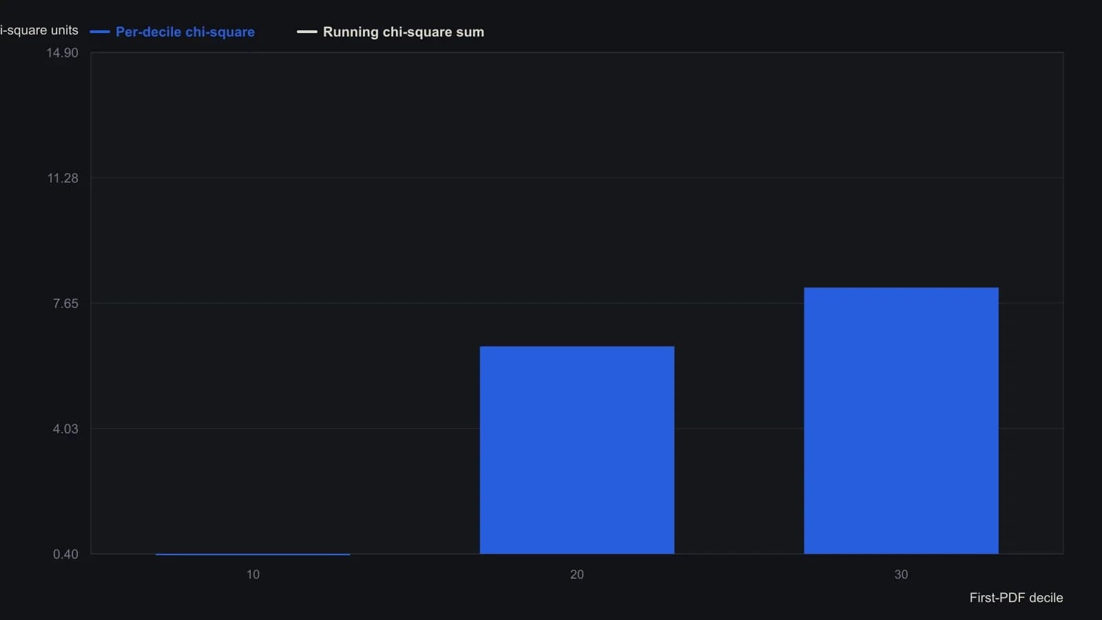
Source uses E = 10 for each decile step and 8 degrees of freedom; chi-square of 15.51 or more rejects stationarity (or, after a stationarity pass, randomness). Only the first three printed rows are recovered; remaining deciles are shown as ellipses and were not invented.
Treat independence as a finite temporal window
Independence is evaluated separately from randomness. One session close is described as partly constraining the next open, so the remaining question is how many sampling intervals that serial influence lasts. That span is the temporal window: the sampling intervals over which serial dependence is still treated as present.
Editorial interpretation: after the stationarity gate and the randomness comparison, leftover serial influence is a finite sampling window, not a market creed.
All readings on this track · 6 readings
- 1986Evaluate the price random-walk question as a gated quantile lab
- 1989Path quantiles versus net return for index velocity regimes
- 1992Opening-referenced percentile stops for same-session gaps
- 1995Read one equity position on a joint yield-regime card
- 2012Construct a pairs-trading worksheet from residuals and quantile ranks
- 2015Constructing mean, median, and mode from ordered prices