2006issue C051-4
Percent-scale average true range for comparable range
Average true range scores amplitude over a lookback, yet the unscaled series stays in price units and mixes range with price-level growth. Dividing that average by a current price restates the same lookback as a percent, so one construction can mark a historical-volatility regime, test whether quiet is unusual, and feed an exposure decision.
- Average true range scores the amplitude of price movement over a lookback, not the directional bias of that movement.
- Unscaled average true range remains in price units, so a higher-priced instrument prints a larger reading and two series cannot be compared directly.
- A normalized average true range divides the same average by a current price such as the latest close or a moving average, restating range as a percent of that divisor.
- The percent-scale series can be lined up against earlier compression troughs as a historical-volatility baseline and used for a cross-market rank before exposure is chosen.
Amplitude over a lookback
Average true range is built to score the amplitude of price movement over a lookback, not the directional bias of that movement. True range for a bar is the largest of the bar high minus bar low, the bar high minus the prior close, and the prior close minus the bar low. Average true range is the average of those true-range values over a fixed lookback, with fourteen a common default, and that average is still expressed in price units.
Price-level bias in the unscaled reading
Unscaled average true range stays in price units, so a higher-priced instrument is expected to print a larger reading than a lower-priced one and the two series cannot be compared directly. That mechanical lift is price-level bias: the unscaled range statistic rises simply because the instrument trades at a higher price.
A percent of a current price
A normalized average true range is constructed by dividing average true range by a current price such as the latest close or a moving average, which restates the range as a percentage of that divisor. When the underlying price changes little over a short sample, the percent-scale plot stays close to the unscaled plot. The two diverge once the price level itself has moved a lot.
A long monthly comparison
On a monthly equity-index study, unscaled average true range sat nearly five times above its level of twenty years earlier while the index itself was about six times higher, so the point series mixed price-level growth with volatility. In the same monthly study, a late-1980s crash produced a percent-scale peak near 13 percent, and that percent series did not retake the crash height until years after the unscaled series had already done so.
A compression trough as a baseline
Because a much higher index level makes a return of unscaled average true range to mid-1990s lows unlikely, the percent-scale series is the construction that can still be lined up against those earlier troughs as a historical-volatility baseline. A historically low percent-scale range reading is a compression trough, used as a baseline for whether current quiet is unusual.
A cross-market rank before exposure
Placed on two yen crosses at different price levels, the percent-scale reading showed the sterling pair had been the wider-ranging market in recent months, supplying a common-unit volatility input before an exposure is chosen. That ordering is a cross-market rank: candidate instruments ordered by percent-scale range so exposure can be chosen on a common volatility unit.
S&P 500 monthly normalized ATR, 1983–2006
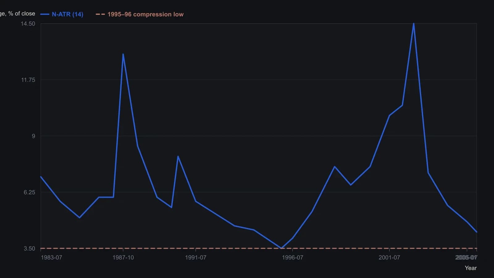
MetaStock construction is ATR(14) divided by the close, times 100, on monthly bars of the S&P 500 continuous contract. The path is digitized from Figure 3; the near-13 percent 1987 peak, the 4.34 percent last print, and the 0.80 percent gap to the mid-1990s low are the levels the article states. Intermediate points are approximate.
When the scaling step matters
The scaling step is described as adding little for a short-horizon desk that watches one instrument. It is the relevant construction when the task is a longer history or a multi-market comparison.
All readings on this track · 6 readings
- 1994Constructing hourly index futures lattices from live volatility
- 1995A short-to-long historical-volatility ratio as a regime-gate
- 2001Constructing a variable-interval average from a difference-oscillator or volatility forecast
- 2006Percent-scale average true range for comparable range
- 2007Historical compression and implied slope as a futures regime map
- 2013GARCH and a volatility rank as market-regime classifiers