1995issue C011-11
Optimal f as a leverage bound for commodity account growth
This archive article separates risk, exposure, and leverage, then treats a growth-maximizing fraction from a consistent track-record sample as a reference bound only. A lower ideal L is the working choice. Monte Carlo reshuffles of completed trades show how sequence can change the equity path.
- Risk is the chance of losing, while exposure is the amount that can be won or lost. Leverage scales that exposure and is not the futures margin deposit.
- Leverage analysis needs a consistent sample of at least 30 completed trades from one mechanical system and one market. Mixed markets, pyramiding steps, or mid-sample system tweaks confound the result.
- The growth-maximizing leverage is only a reference bound. The working choice is a lower ideal L that fits the trader's taste for exposure.
- If that growth-maximizing leverage is at or near zero, revise the system rather than raise leverage. Recalculate ideal L only periodically from a long-run average.
Risk, exposure, and leverage
Risk is the chance of losing on a trade or a sequence of trades. Exposure is the dollar amount that can be won or lost on a position. Leverage is the control that scales exposure. It is not the futures margin deposit.
Commodity leverage is full contract liability divided by account equity: L equals N times P divided by E. Two S&P 500 contracts at 125000 each against 100000 equity give L of 2.5.
Leverage is also a compound-growth choice
Compound growth of equity with full reinvestment multiplies successive one-plus-return factors. Leverage choice is therefore a growth decision as well as a loss-size decision.
Return on equity equals leverage times the raw price change of the contract. The same 5 percent raw move becomes 12.5 percent with L of 2.5. A loss scales by the same factor.
Use one consistent track-record sample
Leverage analysis needs a consistent sample of at least 30 completed trades from one mechanical system and one market. Mixed markets, pyramiding steps, or mid-sample system tweaks confound the result.
That track-record sample of completed trades is the only input used here for leverage and simulation work.
Treat optimal f as a reference bound
The first worksheet search for a growth-maximizing leverage, shown out to a factor of 9.6 on a 30-trade series, is only a reference bound. Optimal f is the leverage or fraction of equity that maximizes compound growth of a fully reinvested trading record.
The working choice is a lower ideal L. Ideal L is selected at or below that growth-maximizing level to match personal tolerance for exposure, not to chase the single highest growth path.
Monte Carlo tests sequence risk
Monte Carlo simulation reshuffles the same completed trades because the next result is random even when expectation is positive. Serial correlation is treated as already absorbed into the system, so the simulations test sequence risk rather than invent new trades.
Recalculate ideal L only periodically
Ideal L should be recalculated only periodically from a long-run average. Updating after every trade, padding results by marking open positions to market, or mixing paper and live rules will skew the bound.
Monte Carlo equity path at four leverages
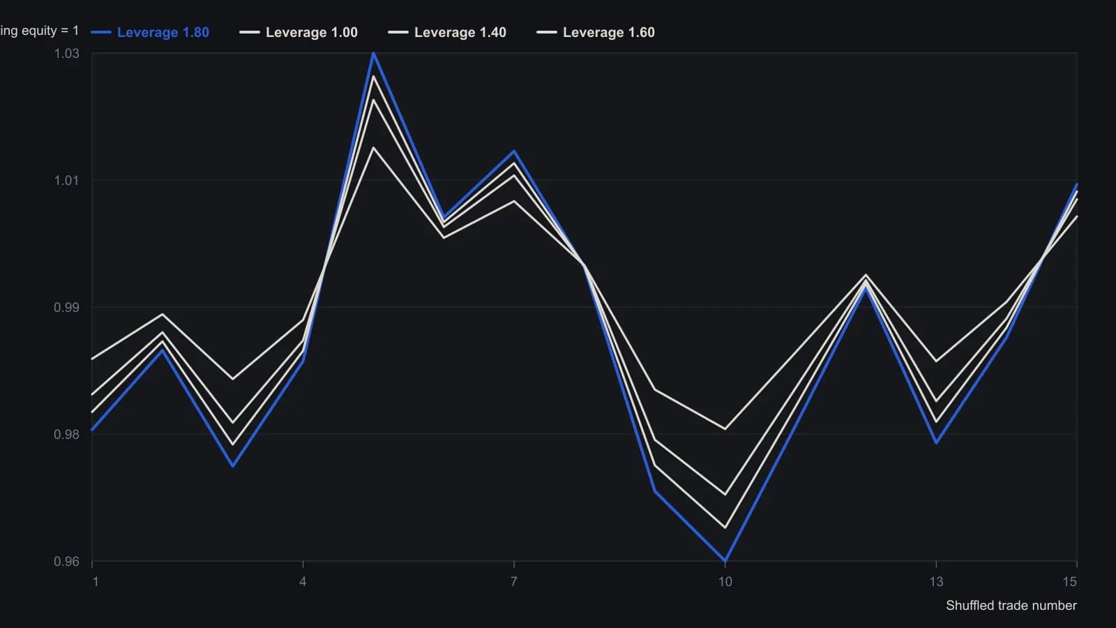
The visible sheet is only the first 15 rows of a 30-trade sample; each probability cell is 0.0333. The article carried leverage as high as 9.6, but this crop stops at 1.80.
TradersWeek editorial reading
This paragraph is an editorial reading and is not part of the archive workflow. TradersWeek reads the procedure as a way to treat leverage as a pre-trade exposure bound rather than as a margin setting. First estimate the growth-maximizing fraction from a consistent track-record sample. Then choose a more conservative ideal L. Monte Carlo paths then show how random sequencing can change, or erase, the equity path even when the same average edge is kept.
All readings on this track · 12 readings
- 1990Constructing optimal f when trade sizes differ
- 1993Portfolio heat, optimal f, and drawdown limits
- 1994Construct historical-optimum-leverage from one equity-path
- 1995Optimal f as a leverage bound for commodity account growth
- 1998Secure f keeps Optimal f sizing inside a Drawdown limit
- 1998Optimal f contract counts versus equity fractions
- 1999Match futures starting capital to system risk
- 1999Search system inputs together with Optimal f sizing
- 2001Bounded crash risk with capital units and optimal f
- 2002Optimal f sizing and risk of ruin as exposure filters
- 2003Cap ruin and drawdown before optimal-f
- 2006Ruin odds, the Kelly fraction and optimal f as size filters