1996issue C041-6
Log-change regression and binomial outlier clusters as an evaluation pipeline
Editorial: TradersWeek treats a market-move forecast as an evaluation pipeline. Convert levels to log-changes, confirm stationarity and independence, fit a linear baseline of yield changes versus index changes, and only then ask whether a tight residual cluster is rarer than chance.
- Absolute price and yield levels stay close to nearby observations, so they are a poor input for methods that assume a more regular, level-free distribution.
- A log-change converts those levels into a series that can be compared across instruments and that approximates a rate of return over a modest percentage range.
- A stationarity-pretest and a serial-dependency-pretest must come before any forecast is read from the series.
- After a regression-baseline is fitted, a binomial-count-test asks whether an outlier-cluster is more than a chance fluctuation around the line.
From levels to log-changes
Editorial: TradersWeek treats a market-move forecast as an evaluation pipeline rather than as a single reading. The archive describes the historical workflow that follows, beginning with the input series.
Absolute price and yield levels stay close to nearby observations, so they are a poor input for methods that assume a more regular, level-free distribution. Differencing the natural log converts those levels into a log-change series that can be compared across instruments and that approximates a rate of return over a modest percentage range. Successive observations can then be compared without the level of the series dominating the result.
Pretests before any forecast
Before any forecast is read from the series, a stationarity-pretest and a serial-dependency-pretest are required so that later inferences are not drawn from a shifting or auto-repeating process.
The stationarity-pretest places log-changes of the index into mutually exclusive bins, compares first-half and second-half counts, and summarizes the mismatch with a chi-square statistic. That check asks whether the rules generating the series stay stable enough across halves of the sample that later inferences are not driven by a shifting process.
The serial-dependency-pretest asks whether one observation is simply a function of the previous one, so a later test is not counting the same information twice.
Regression baseline and the expected band
After those pretests, a regression-baseline is formed by a linear regression of log-changes in the related yield series onto log-changes in the index. The fitted linear map, here from a Treasury yield onto the target index, defines the band in which later observations are expected to fall. It is used to define an expected band rather than a trade.
Outlier clusters and the binomial count
Residuals outside a 1.96 residual-spread band are treated as outliers. A binomial-count-test then calculates a probability on the number of out-of-band observations in a short window and asks whether that outlier-cluster is consistent with independent chance under the fitted model.
In the supplied sample, a dense cluster of such outliers appeared only in the weeks just before a large late-1994 rise in the index. The evaluation treats that cluster as a candidate break in the fitted rate-index relationship rather than as a standalone signal.
S&P 500 weekly log-change bins, first half versus second half
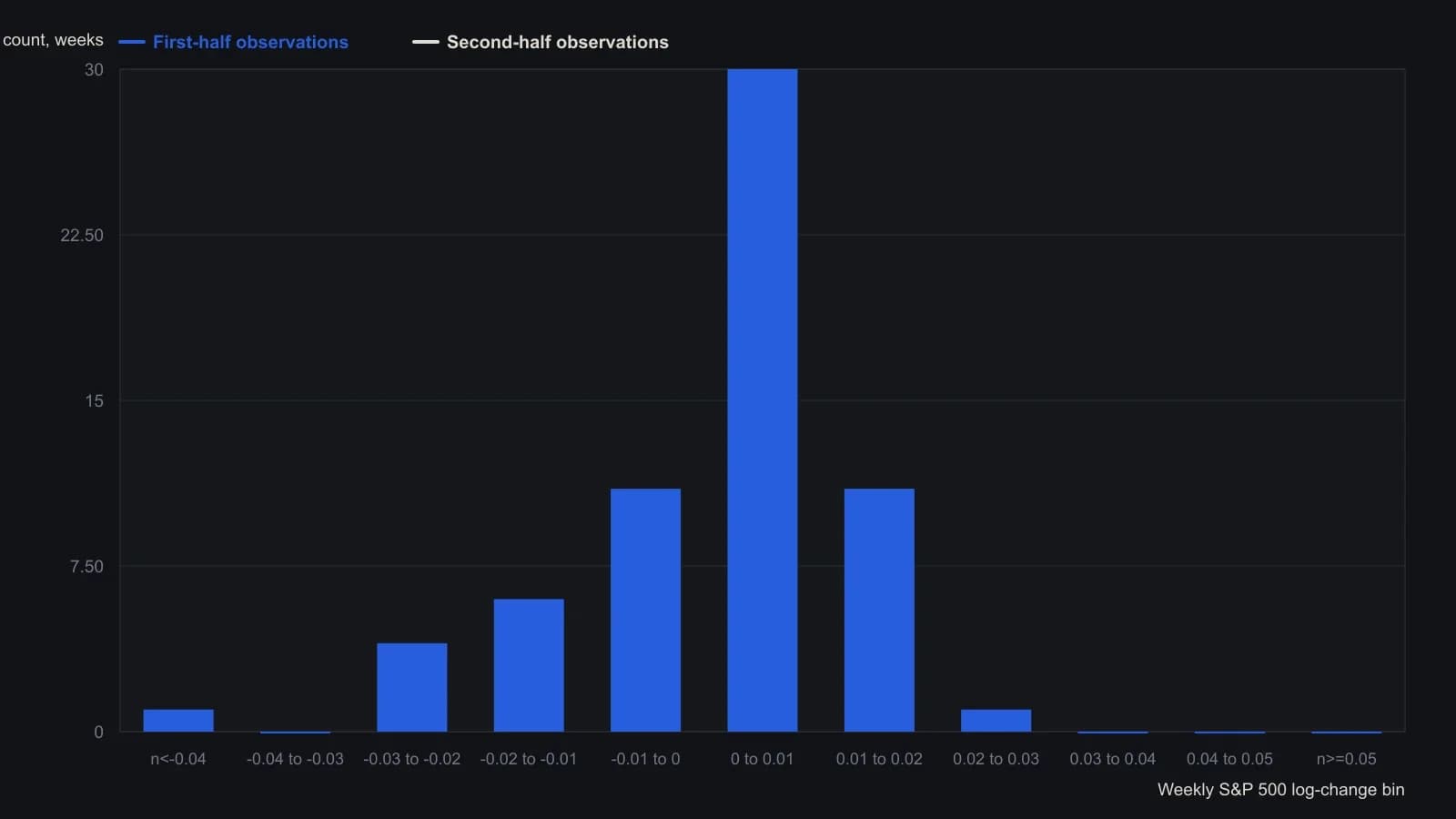
Each half has 64 weekly observations. The author then applied chi-square to the cumulative bin counts (6.891 versus a 18.307 critical value at 10 degrees of freedom) and treated the series as stationary. Only the first five individual deltas are printed; this series uses the article's full-sample totals.
All readings on this track · 7 readings
- 1989Auditing price motifs against binomial chance
- 1991How equal independent stakes change the odds of a complete loss
- 1991Binomial counts for unrelated position construction
- 1996Log-change regression and binomial outlier clusters as an evaluation pipeline
- 1996Constructing a log-change stationarity screen with regression or binomial tests
- 1998Binomial baselines for discount-rate change timing
- 2002Trade-count horizon for equity-curve survival