1989issue C101-9
Auditing price motifs against binomial chance
After any pattern-recognition filter on ordered up and down prints, score the leftover two-outcome count against a binomial chance band. Treat every extra series or calendar window searched as another draw that makes a striking leftover more likely.
- Repeating motifs appear in purely random two-outcome sequences and can closely resemble the historical price motifs recovered by pattern recognition.
- The remaining sample after a prefix or weekday filter is the proper denominator for a continuation rate, and relative variation grows as that leftover shrinks.
- Search multiplicity across series, prefixes, or calendar windows raises the chance that at least one leftover looks unusual.
- Mapping ordered up and down prints onto a multi-year calendar window does not, by itself, show that those prints differ from random binary data.
A pre-forecast audit
Pattern recognition is scanning ordered price, volume or breadth prints for repeating motifs and treating a high next-step rate as a forecast. Repeating motifs appear in purely random two-outcome sequences and can closely resemble the historical price motifs recovered by pattern recognition.
Editorial: TradersWeek treats that continuation rate as a pre-forecast audit, not as a finished forecast. After any pattern-recognition filter on ordered up and down prints, score the leftover two-outcome count against a binomial chance band.
What a binomial count allows
A binomial probability model is a two-outcome counting model whose expected frequency is the trial count times the event chance and whose spread around that count grows with the trial count even as the relative spread shrinks. Under that model the typical absolute spread around an expected pattern count grows with the number of trials, while that spread as a share of the mean shrinks.
For 400 trials of a four-step motif with chance 1/16, the expected count is 25 and the standard deviation is about 4.8, a relative spread of about 19%. In one 16-motif coin-toss histogram, 8 frequencies sat inside one standard deviation of the mean, all 16 sat inside two, and none landed exactly on the mean.
Four-toss frequencies versus the binomial chance band
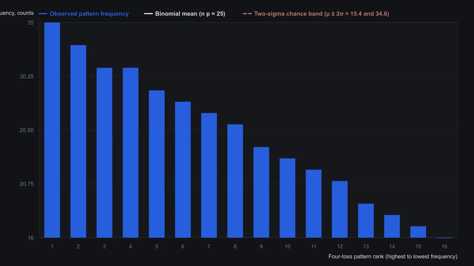
n = 400 independent four-toss trials; each of the 16 equally likely patterns has mean frequency 25 and standard deviation about 4.8. Bars are the same simulation as Figure 1, reordered highest to lowest. Digitized from the printed histogram; individual heights are approximate to the nearest count.
Why leftover rates look large
Conditioning on longer prefixes shrinks the leftover sample, so a 65% next-step rate after a three-toss motif can appear in random data and is visible in a subsequence breakdown. The remaining sample is the much smaller count of cases left after a prefix or weekday filter, which is the proper denominator for a continuation rate. Relative variation is the size of a frequency swing compared with its expected count; this share grows as the leftover trial count shrinks. Relative imbalance between the two outcomes grows as the remaining trial count shrinks.
After a five-step filter the leftover samples were about 43 to 63 trials, with a mean near 54.7, so a swing of about 15 percentage points is near two standard deviations and is expected among 32 prefixes. An unconditional 60% Monday down-close rate over 400 weeks is a much rarer chance event than a 60% Friday down-close rate after four up days, because the second claim may rest on only about 25 leftover cases and overlapping multi-day windows are not independent.
Many searches, one striking leftover
Search multiplicity is the number of series, prefixes or calendar windows inspected; more searches raise the chance that at least one leftover looks unusual. Repeating the search many times makes at least one striking leftover more likely.
In 20 simulated series of 1,750 six-toss trials, all but two series produced at least one five-toss prefix whose sixth toss cleared a 65% or 35% cutoff, even though a few leftover subsequences can pull those rates. Mapping 400 observations onto eight years of Tuesday-through-Friday up/down prints does not, by itself, show that those ordered prints differ from random binary data.
Editorial: treat every extra series or calendar window searched as another draw that makes a striking leftover more likely.
All readings on this track · 7 readings
- 1989Auditing price motifs against binomial chance
- 1991How equal independent stakes change the odds of a complete loss
- 1991Binomial counts for unrelated position construction
- 1996Log-change regression and binomial outlier clusters as an evaluation pipeline
- 1996Constructing a log-change stationarity screen with regression or binomial tests
- 1998Binomial baselines for discount-rate change timing
- 2002Trade-count horizon for equity-curve survival