2001issue C061-6
How a fixed smoother becomes a living parameter surface
A conventional filter cannot retune when the trend character of a series changes. Substituting least-squares r-squared for a fixed amplification lets Exponential smoothing set its own gain while the period stays short. The historical workflow then asks whether nearby settings still behave, and treats any working set as valid only for a finite interval.
- A conventional filter keeps its fitting constants fixed for every observation, so it cannot retune itself when the trend character of the series changes.
- Least-squares r-squared, which runs from 0 for no fit to 1 for a perfect fit, can replace a fixed sensitivity constant so the Adaptive Filter learns its own gain from the data.
- Parameter-surface inspection treats orderly slopes from a period of 2, and the absence of isolated peaks once sensitivity exceeds 10, as signs that a setting is not a lone spike.
- A working parameter set is valid only for a finite interval and is meant to be rechecked by watching rank movement of results.
Fixed constants cannot follow a changing trend
A conventional filter keeps its fitting constants fixed for every observation, so it cannot retune itself when the trend character of the series changes. Exponential smoothing still needs an explicit gain. Least-squares r-squared, which runs from 0 for no fit to 1 for a perfect fit, can replace a fixed sensitivity constant so the smoother learns its own gain from the data.
A short lookback with a learned gain
The baseline smoother is built by cubing an amplified two-term average. Successive exponential averages of the close, with alpha equal to 2 divided by period plus one, are combined with coefficients that depend on an amplification factor a between 0 and 1.
Default construction of that smoother uses period 5 and amplification 0.7. The Adaptive Filter keeps the period in a short band, typically 2 to 12, and substitutes r-squared for the fixed amplification.
Five-period T3: sample close and first exponential average
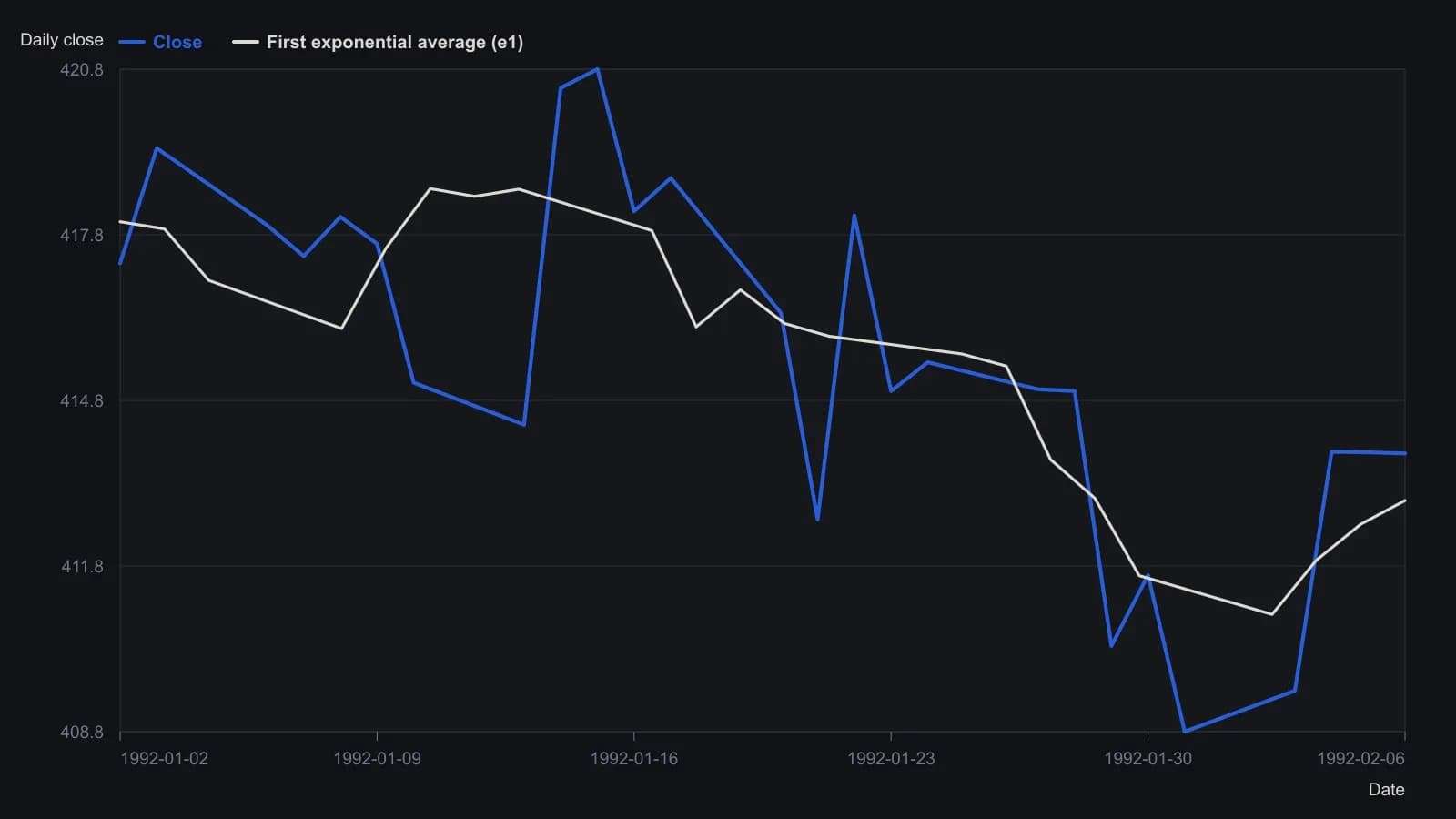
Period is fixed at 5 and the volume factor a at 0.7. Six nested exponential averages must fill before T3 prints, so the sheet shows only the first two T3 values and no adaptive r-squared yet.
Entry, exit and reversal as one procedure
The tested procedure is a complete long-short rule: enter long when close falls below the filter and enter short when close rises above it, so entry, exit and reversal are one testable system. System optimization is what makes those rules testable as one procedure.
A reported nonadaptive calibration used period 12 and sensitivity 2. On that same series the adaptive substitution changed both the trade count and the reported profit-loss and reward-risk indexes relative to the fixed-parameter run.
Nearby settings decide whether a peak is usable
Parameter-surface inspection is part of the method. Slopes that remain orderly from a period of 2, and the absence of isolated peaks once sensitivity exceeds 10, are treated as signs that a setting is not a lone spike.
The same historical workflow can show a strong equity window and then a plateau. A working parameter set is described as valid only for a finite interval and is meant to be rechecked by watching rank movement of results.
A fast weekly operating envelope
The proposed operating envelope keeps the filter fast by holding period and sensitivity below 10, prefers a weekly bar so a trend can form, and limits each name to a small share of its five-period average volume.
Reported equity paths assume no interest, taxes, commissions or margin. A perfect-hindsight weekly long-short path is shown only as an upper bound on what frequent position changes could extract, not as a live result.
All readings on this track · 9 readings
- 1982Constructing moving averages with weights, alignment, and adaptive lookbacks
- 1990Constructing adaptive filters from equal-weight averages
- 2000Cycle-scaled lookbacks for a channel-breakout rule
- 2000When charting code breaks the adaptive trendline
- 2001Nonlinear Ehlers filter construction from momentum and distance weights
- 2001How a fixed smoother becomes a living parameter surface
- 2005A three-part workshop for adaptive-filter length search
- 2010Rebuilding an exponential average as a bounded error-correcting filter
- 2018Assembling a recursive median oscillator as a two-stage adaptive filter