1989issue C031-7
Smoothing filters, cutoff, poles, and sample delay
A smoothing filter keeps lower-frequency variation in an ordered price series and reduces high-frequency jitter. Extra poles can sharpen the cutoff, but each pole adds filter delay, so a moving average or a one-state exponential smoother remains the ordinary construction.
- A smoothing filter keeps lower-frequency variation and reduces high-frequency jitter. An exponential smoother does this with a recursive one-state update that stores only the last output.
- Extra poles steepen attenuation toward a near-brick-wall cutoff, and each added pole adds a sample of filter delay.
- A finite-window moving average and a recursive exponential smoother have similar amplitude responses. The moving average is treated as adequate because it is simplest and introduces the least delay.
- A higher-pole Butterworth output can be smoother than a matched exponential smoother, but the extra lag and construction complexity are judged not justified for ordinary smoothing.
What a smoothing filter keeps
A smoothing filter is built to keep lower-frequency variation in an ordered price series and reduce high-frequency jitter. An exponential smoother does this by attenuating rapid changes while retaining slower ones.
A one-state exponential update
An exponential smoother is recursive. The current output equals a fraction of the current observation plus one minus that fraction times the previous output, so only the last output needs to be stored.
With a unit-delay operator, the exponential-smoother transfer response equals one when delay is zero, so a constant input passes unchanged. The same response has a pole where the denominator is zero.
Poles, cutoff, and transfer response
Extra poles steepen attenuation toward a near-brick-wall cutoff. A two-pole transfer response is a second-order ratio whose denominator has two roots. Successive pole counts approach that sharp cutoff when curves are aligned at the half-power amplitude of 0.707.
Frequency is the reciprocal of cycle period, so a 10-day cycle is 0.1 cycles per day. A 10-day single-pole design maps roughly to a 2.1-day exponential smoother, and a 20-day single-pole design maps to a 4.2-day exponential smoother.
Butterworth amplitude vs poles
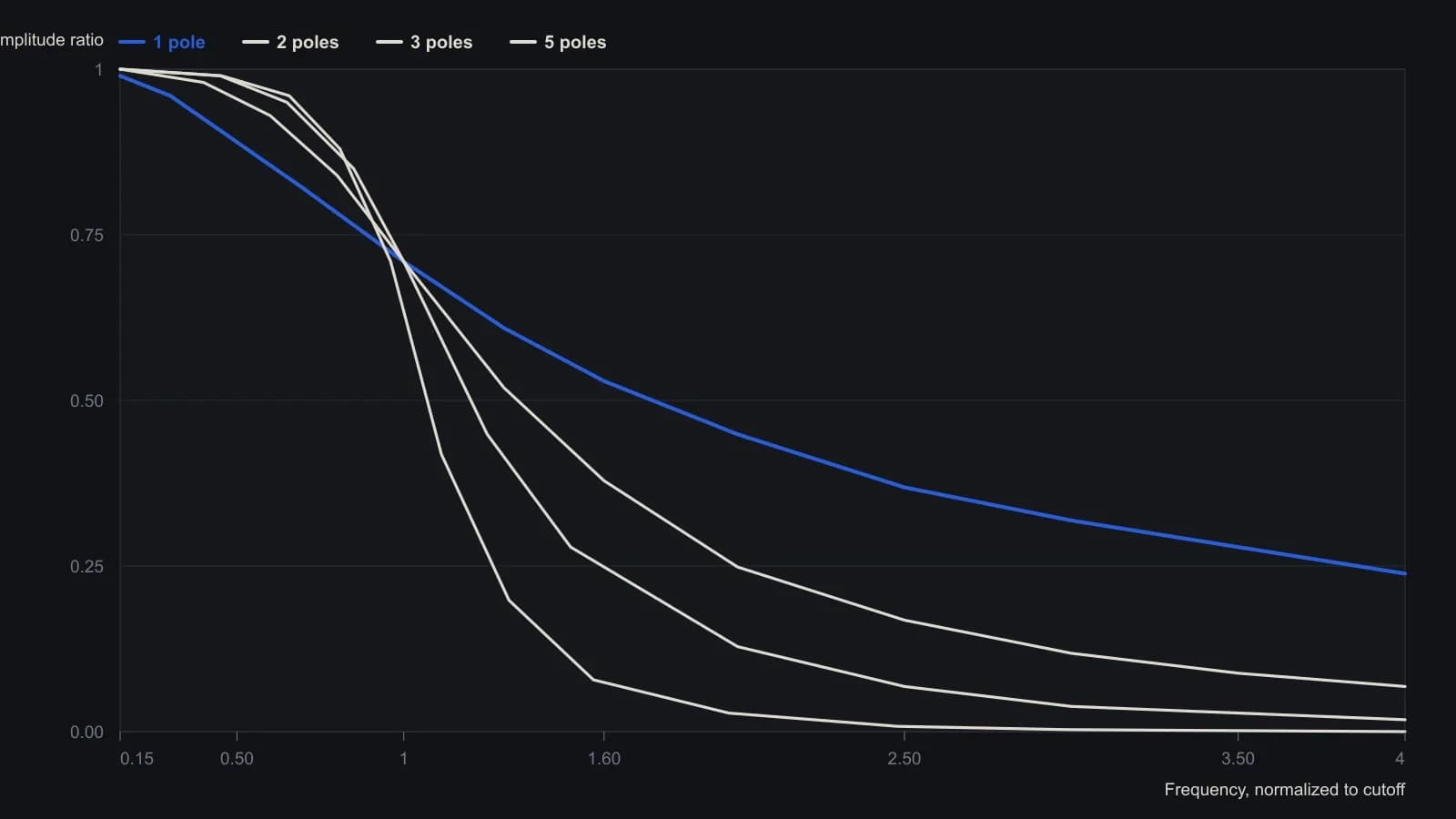
Curves are normalized to cutoff so half-power bandwidth equals 0.707 wave amplitude. Text also states a two-pole filter is about 0.25 amplitude at twice cutoff.
Delay from extra poles
Each added pole adds a sample of delay. A five-pole design has five delay stages. Butterworth low-frequency delay of about N times the cutoff period over pi squared is nearly five days for a five-pole filter with a 10-day cutoff, and delay nearly doubles near cutoff.
A Bessel-type response cuts that delay by about half. A three-pole Bessel design with a 20-day cutoff delays about three days, while a 7-day exponential smoother delays a little more than one day and has a similar amplitude curve.
A 20-day three-pole Butterworth output is smoother than a 7.44-day exponential smoother but with substantially more lag, so the extra construction complexity is judged not justified for ordinary smoothing.
Why the simple window stays enough
A finite-window simple moving average is a finite impulse response filter: the output depends on a finite window of past observations and has no stored-output feedback. That moving average and a recursive exponential smoother have similar amplitude responses by construction. The exponential form usually lags slightly less because older observations are down-weighted instead of equally included.
A moving average is treated as adequate smoothing because it is simplest to implement and introduces the least filter delay, leaving simple versus exponential form as a designer choice. Several filters that share one cutoff but differ in pole count would stagger in time and could be differenced into a lead, at extra construction cost.
All readings on this track · 10 readings
- 1982An odd-length smoother from a cycle cutoff
- 1989Smoothing filters, cutoff, poles, and sample delay
- 1992Constructing a cycle-aware finite impulse response detrender
- 2002Rebuild a smoother by writing the lag into the coefficients
- 2002Timing market cycles with finite impulse response filters and FFT
- 2002Constructing the relative strength index with an even-order finite-impulse-response prefilter
- 2003Recursive and cascaded moving-average construction
- 2006One second-order transfer function, a family of trend filters
- 2019Constructing the Voss line from a bandpass and a short FIR sum
- 2020Truncated bandpass construction as a finite-length trend filter