1990issue C101-16
Constructing a short-horizon ARIMA from differenced wheat closes
A wheat close series is differenced only after its autocorrelation plot refuses a stable mean. Residual autocorrelation, not a high in-sample fit, then decides which short p, d, and q triple may emit the next close.
- Differencing is applied after slowly decaying autocorrelations on the raw closes show that a constant mean is unrealistic.
- Partial autocorrelations that start near one and then fall toward zero favor a short autoregressive skeleton, with both autoregressive and residual lags kept at or below three days.
- Large coefficient t-statistics and an in-sample R-squared near 98.7 percent do not keep a specification if leftover residual correlation still rejects it.
- Only the first-differenced form with one autoregressive lag and two residual lags is accepted for the one-step close update.
A one-step close as a short weighted sum
In this construction, ARIMA is a one-step close forecast built from a few lags of the possibly differenced series plus a few lags of leftover forecast residuals. A one-step wheat-close forecast can be assembled as a short weighted sum of recent transformed prices and recent forecast residuals, where the series is either the raw close or its first difference.
Difference after the mean fails
A constant-mean assumption is treated as unrealistic for that wheat series, so the construction first replaces each close with its change from the prior close. Differencing means replacing each close with its change from the prior close so a trending series can be treated as having a more stable mean.
Slowly decaying sample autocorrelations on the undifferenced closes are used as the identification signal that one difference is required.
CBOT wheat close autocorrelations fade too slowly to treat the mean as fixed
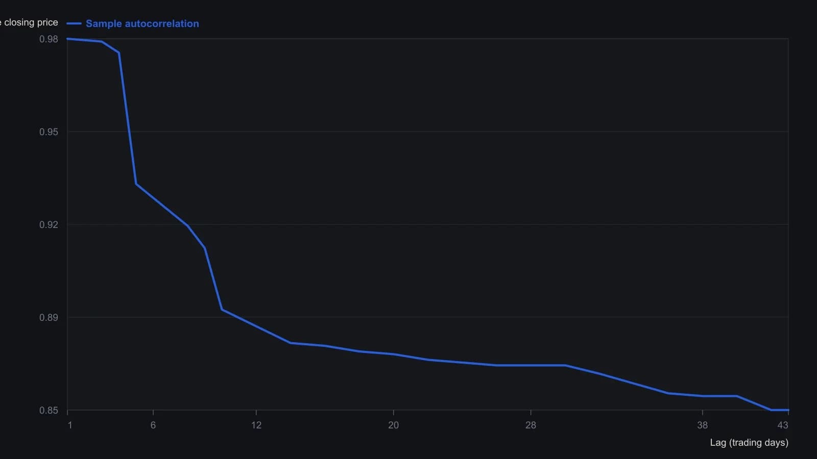
1,054 CBOT wheat closes from 3 July 1983 through 30 July 1987. Lags whose printed coefficients were not legible on the scan are omitted; missing lags are not interpolated.
A short autoregressive skeleton
An autocorrelation test reads lag-by-lag and partial correlations to choose p, d, and q, then checks leftover residual correlation to keep or discard that choice. A partial autocorrelation is the correlation between closes a given number of days apart after the influence of the intervening days has been removed.
Partial autocorrelations that start near one and then fall toward zero are used to prefer a short autoregressive skeleton, and both the autoregressive and residual-lag lengths are kept at or below three days.
On 1,054 daily wheat closes, a 99 percent Quenouille band of -0.079 to 0.079 is applied to the partial autocorrelations, and a third-lag reading outside that band is the reason p=1 and p=3 are both estimated. That Quenouille band is a large-sample interval around zero used to judge whether a partial autocorrelation at a given lag is distinguishable from noise.
Residual checks reject the level fits
An undifferenced one-lag level fit produces coefficient t-statistics of 278.74 and 12.42, both above the 2.575 cutoff used at 99 percent for large samples, yet residual Ljung-Box-Pierce statistics still reject that specification. A Ljung-Box-Pierce check asks whether leftover dependence is still large enough to reject the specified p, d, and q.
A second autoregressive lag fails a zero-coefficient t-test, and a three-lag autoregressive alternative keeps every lag, but residual autocorrelation still rejects both undifferenced candidates.
The only accepted triple
Across the p, d, and q combinations that were estimated, only the first-differenced specification with one autoregressive lag and two residual lags is accepted by the Ljung-Box-Pierce residual test.
After that first difference, the retained one-step update is the latest close plus 0.5111 times the latest daily change plus 0.4924 and 0.1260 times the two most recent residual errors, and the intercept is dropped after a 99 percent t-test. Those residual errors are disturbances: the part of today's transformed price that is not explained by the model's own past prices or past residuals.
Fit describes, it does not certify
In-sample R-squared near 98.7 percent is reported for several differenced candidates and is treated as a fit description only, not as proof that a specification is statistically adequate.
As an editorial reading, a high in-sample fit is not a reason to emit the next close. Residual autocorrelation remains the keep-or-discard rule.
All readings on this track · 6 readings
- 1982Construct ARIMA forecasts from lag diagnostics
- 1985Evaluating ARIMA envelopes as entry, exit and stop rules
- 1985Daily ARIMA range as a filter for intraday stochastic divergence
- 1990Constructing a short-horizon ARIMA from differenced wheat closes
- 2014ARIMA earnings forecasts versus the announcement-window price reaction
- What an early ARIMA commodity forecast teaches about model limits