1985issue C051-9
Constructing a recursive two-gain price smoother
A recursive two-gain update on evenly sampled prices can be read as a Kalman estimator, an alpha-beta filter, or a lowpass smoother. Editorial reading: change only the gain law and the sampling interval.
- Even sampling is required. A continuous price path is treated as discrete samples taken at a fixed interval so the filter math applies.
- One second-order recursion revises the change term with K1 and the smoothed level with K2, then predicts the next sample as that level plus the change term.
- The same update is an infinite-impulse-response lowpass filter. Lowering the filter factor removes more high-frequency content and slides the cutoff.
- A first-order form would hold the level constant. The second-order form updates level and acceleration, and a large residual can raise K1 so the filter recaptures faster.
Price smoothing as one construction
The construction treats a continuous price path as discrete samples and requires those samples to be taken at even intervals for the filter math to apply. Even sampling means collecting observations at a fixed interval so discrete-time filter constructions remain valid.
Smoothing is defined as attenuating high-frequency components so slower cycles remain. A centered five-observation moving average is the usual time-domain baseline and can respond unevenly to nearby cycle lengths.
One recursive two-gain update
The second-order Kalman construction is a recursive alpha-beta update. The prediction residual equals the measured value minus the predicted value. The change term is revised by K1, the smoothed level is revised by K2, and the next prediction is the smoothed level plus the change term.
The Kalman filter, in this construction, is a recursive estimator that revises a predicted level from evenly spaced observations by folding the latest residual into both the smoothed value and a change term. The alpha-beta filter is the two-gain form of that recursion: one weight updates the change term and the other updates the level, with the second gain often tied to the first by a square-root rule.
Starting values and the companion gain
Initialization sets the first observation as the prediction, the change term to zero, K1 between 0 and 0.5, and K2 to the square root of twice K1. The filter factor is that free gain chosen between 0 and 0.5. It sets how strongly residuals revise the change term and, through the companion gain, the smoothed level.
The same equations as a lowpass filter
The same recursion is an infinite-impulse-response lowpass filter with a predictive term. Each observation influences all later outputs, and that influence decays toward but never reaches zero.
A lowpass filter passes slower cyclic components and attenuates faster ones. Moving the recursive gains slides the cutoff along the frequency axis.
What changes when only the gain law changes
Lowering K1 from 0.25 to 0.10 removes more high-frequency content. A K1 near 0.5 almost follows the raw series and delays it by one sampling interval.
Changing the filter factor slides the lowpass cutoff along the frequency axis. Linear paths are tracked and the next sample is predicted without residual error, while nonlinear motion produces lag.
Level, acceleration, and a jump in K1
A first-order Kalman form would treat the level as constant. The second-order form updates both level and acceleration, and the residual can raise K1 after large jumps so the filter recaptures faster. In the worked example K1 is 0.25 when the residual exceeds 30 points, otherwise 0.12.
Two-gain smoother frequency response at three K1 settings
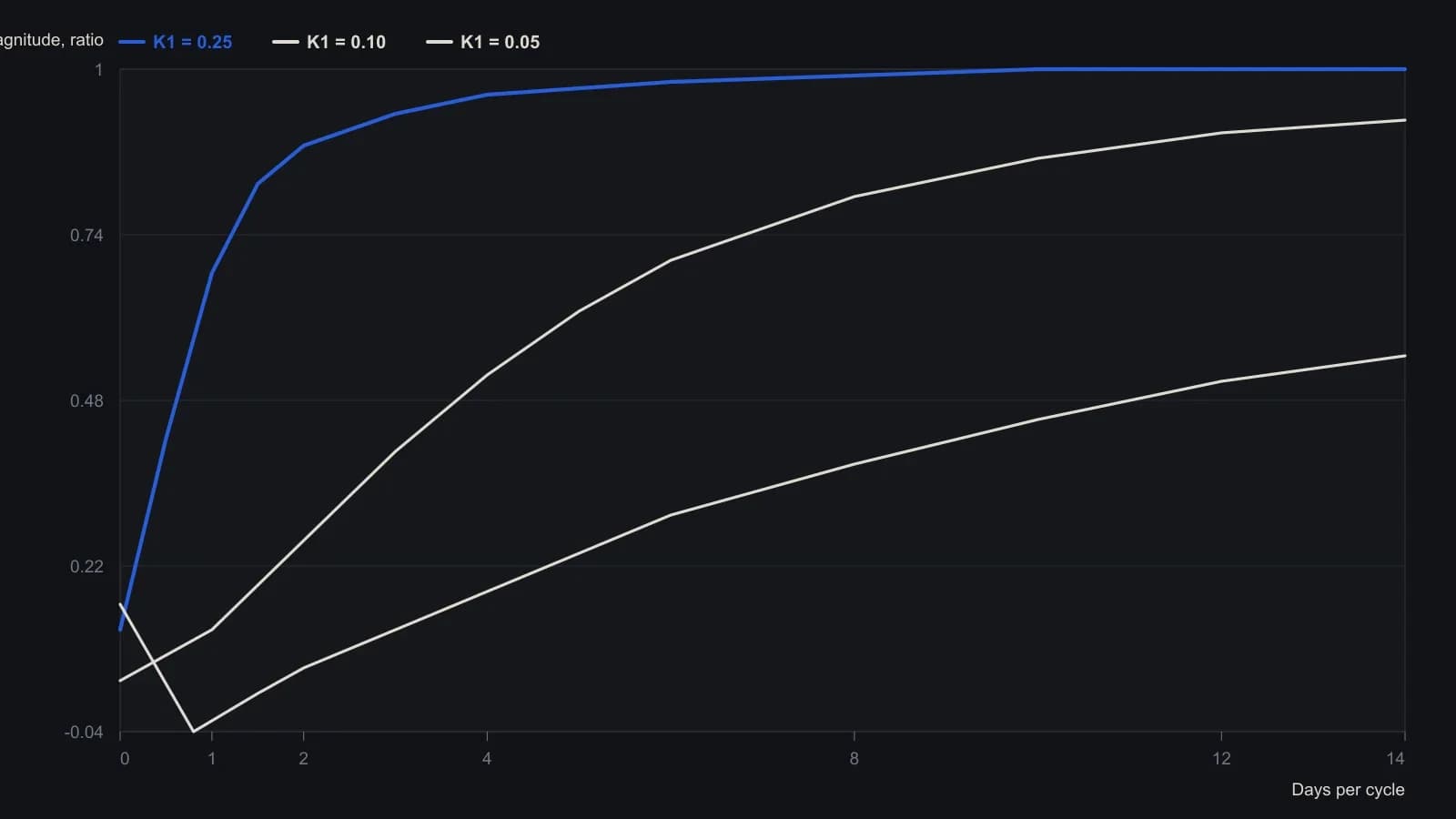
One sample per day, as in the article. The magazine scan is mirrored; series names follow the stated gain law (larger K1 keeps more short-cycle magnitude). Vertical scale is linear magnitude, not log. Points are approximate reads from the raster, not exact Fourier output.
All readings on this track · 7 readings
- 1985Constructing a recursive two-gain price smoother
- 1989Constructing alpha-beta price channels and trend filters
- 1989Alpha-beta lag parameters versus moving-average windows
- 1995Constructing a reproducible alpha-beta price channel
- 2006Shared coefficient construction for recursive price filters
- 2010How to judge a Kalman filter forecast as a Trend filter
- 2019Constructing a calendar-conditioned trend filter